Processing with HDF5 datasets#
Unlike the h5py package, which returns numpy.ndarray when accessing the values of datasets, the h5rdmtoolbox returns xarray.DataArray objects. The xarray.DataArray object allows to carry attributes with the numpy-like multi-dimensional array. It also supports the concept of dimensions and coordinates, allowing to assign the array axis with meaning ful (meta) data.
Let’s dive into it and explore the practical implications of retrieving xarray.DatArray:
import h5rdmtoolbox as h5tbx
import numpy as np

h5tbx.use(None)
using("h5py")
Let’s create an example file. Note, that we pass make_scale and attach_scale as arguments to setup the coordinates and their association to the HDF5 dataset “data”. The useful implications will be visible when we access the dataset values in the next steps.
with h5tbx.File() as h5:
    dsx = h5.create_dataset('x', data=np.linspace(0, 10, 5),
                            attrs=dict(units='mm', long_name='x'),
                            make_scale=True)
    dsy = h5.create_dataset('y', data=np.linspace(0, 5, 11),
                            attrs=dict(units='mm', long_name='y'),
                            make_scale=True)
    h5.create_dataset('vel', data=np.random.random((11, 5)),
                      attrs=dict(units='m/s', long_name='velocity'),
                      attach_scales=(dsy, dsx))
    h5.dump()
-
-
(y: 11, x: 5) [float64]
- long_name: velocity
- units: m/s
-
(5) [float64]
- long_name: x
- units: mm
-
(11) [float64]
- long_name: y
- units: mm
Array Slicing#
Slicing an HDF5 dataset returns a xarray.DataArray
with h5tbx.File(h5.hdf_filename) as h5:
    data = h5.vel[:]
data
<xarray.DataArray 'vel' (y: 11, x: 5)> Size: 440B
0.1065 0.9509 0.1665 0.4592 0.6336 0.6975 ... 0.1911 0.1856 0.1333 0.9659 0.3978
Coordinates:
  * y        (y) float64 88B 0.0 0.5 1.0 1.5 2.0 2.5 3.0 3.5 4.0 4.5 5.0
  * x        (x) float64 40B 0.0 2.5 5.0 7.5 10.0
Attributes:
    long_name:  velocity
units: m/sAdvantages of retrieving xarray.DataArray#
Few of the advantages:
attributes (aux. info) with the array
.attrs(copied from the HDF dataset to thexarray.DataArray)dimensions and coordinates (1D arrays) to address the axis by label rather than by idex
apply operations (computations, visualizations) based on the meta data
data.attrs
{'long_name': 'velocity', 'units': 'm/s'}
Select subarray by specifying coordinate values for a given axis (coordinate):
data.sel(y=2.0)
<xarray.DataArray 'vel' (x: 5)> Size: 40B
0.1528 0.2291 0.1331 0.06862 0.1843
Coordinates:
    y        float64 8B 2.0
  * x        (x) float64 40B 0.0 2.5 5.0 7.5 10.0
Attributes:
    long_name:  velocity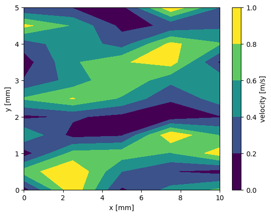
units: m/sPlot data by using information from attributes and coorinates:
data.plot.contourf()
<matplotlib.contour.QuadContourSet at 0x796834e9b430>
Selecting data (.sel)#
HDF5 datasets may sometimes be very large. Hence it is ineffcient to slice a larger array and then use the useful method of (selecting)[https://docs.xarray.dev/en/stable/user-guide/indexing.html]. The h5rdmtoolbox allows to call .sel prior to the above slicing, to reduce the data loaded to the RAM:
with h5tbx.File(h5.hdf_filename) as h5:
    print('available coords to select from: ', h5.vel.coords.keys())
    xdata = h5.vel.sel(y=2.0)
xdata
available coords to select from: dict_keys(['y', 'x'])
<xarray.DataArray 'vel' (x: 5)> Size: 40B
0.1528 0.2291 0.1331 0.06862 0.1843
Coordinates:
    y        float64 8B 2.0
  * x        (x) float64 40B 0.0 2.5 5.0 7.5 10.0
Attributes:
    long_name:  velocity
units: m/sHDF Dataset with ancillary datasets#
Ancillary datasets, which exist in the HDF5 file and are associated to one dataset. The ancillary datasets must have the same shape as the parent dataset.
An common use-case is the association of validation flags or uncertainty data.
Let’s add a relative uncertainty of 5% to the dataset “vel”. For this we create the dataset “uncertainty” and attach it to the already existing dataset “vel”:
rel_uncertainty = np.clip(np.random.normal(loc=0.025, scale=0.001, size=(11, 5)), 0, None)
with h5tbx.File(h5.hdf_filename, mode='r+') as h5:
    h5.create_dataset('uncertainty',
                      data=rel_uncertainty,
                      attach_scales=('y', 'x'),
                     attrs={'units': ''})
    h5.vel.attach_ancillary_dataset(h5.uncertainty)
h5tbx.dump(h5)
-
-
(y: 11, x: 5) [float64]
- units:
-
(y: 11, x: 5) [float64]
- long_name: velocity
- units: m/s
-
(5) [float64]
- long_name: x
- units: mm
-
(11) [float64]
- long_name: y
- units: mm
The ancillary dataset will appear as a xarray coordinate when the dataset is sliced:
with h5tbx.File(h5.hdf_filename) as h5:
    u = h5.vel[()]
with h5tbx.File(h5.hdf_filename) as h5:
    print('available ancillary datasets: ', h5.vel.ancillary_datasets)
    data = h5.vel.sel(y=3.1, method='nearest')
data.coords
available ancillary datasets: {'uncertainty': <HDF5 dataset "uncertainty": shape (11, 5), type "<f8", convention "h5py">}
Coordinates:
    y            float64 8B 3.0
  * x            (x) float64 40B 0.0 2.5 5.0 7.5 10.0
    uncertainty  (x) float64 40B 0.02671 0.0231 0.02527 0.02485 0.02642
Unit interface#
It is reasonable to provide physical units to the datasets. This is probably one of the most important meta information about a dataset. You might have noticed its usage in the examples above.
If the dataset is sliced as is, the returned xarray.DataArray will have the respective unit. In some cases, it might be necessary to convert the data (and/or its coordinates) into another unit. The h5rdmtoolbox provides an interface for this purpose. Address the desired dataset and call to_units(...) on it, which will call the interface class. The latter implements all major methods, like sel, isel and __getitem__.
Note, that this feature must be “enabled” by importing the units modue from extensions. The implementation principle is discussed here.
from h5rdmtoolbox.extensions import units
with h5tbx.File(h5.hdf_filename) as h5:
    data = h5.vel.to_units('mm/s', x='m')[()]
data
<xarray.DataArray 'vel' (y: 11, x: 5)> Size: 440B
106.5 950.9 166.5 459.2 633.6 697.5 ... 350.6 191.1 185.6 133.3 965.9 397.8
Coordinates:
  * y            (y) float64 88B 0.0 0.5 1.0 1.5 2.0 2.5 3.0 3.5 4.0 4.5 5.0
    uncertainty  (y, x) float64 440B 0.02529 0.02295 0.02548 ... 0.02513 0.02325
  * x            (x) float64 40B 0.0 0.0025 0.005 0.0075 0.01
Attributes:
    ANCILLARY_DATASETS:  ['uncertainty']
    long_name:           velocity
units: mm/sAs a side note, xarray works well with pint, which is a units-library. Please refer to the pint-xarray documentation or to this blog entry about it for detailed explanation and #examples on how it is done.
The following shows an example usage of it (which takes place under the hood of to_units() implemented in the h5rdmtoolbox:
# note, that we need to call the "pint"-accessory every time to make the xarray object
quantified_data = data.pint.quantify(unit_registry=h5tbx.get_ureg())

u_mm_s = quantified_data.pint.to('mm/s').pint.dequantify()
u_mm_s.units
'mm/s'