Visualization

As the return value of a sliced dataset is a xarray.DataArray instead of a numpy.ndarray plotting features of xarray is used. For more information about xarray see https://docs.xarray.dev/en/stable/

import h5rdmtoolbox as h5tbx
h5tbx.use(None)

import matplotlib.pyplot as plt
import numpy as np

Failed to import module h5tbx

with h5tbx.File() as h5:
    dsx = h5.create_dataset('x', data=np.linspace(0, 10, 20), attrs=dict(units='mm', long_name='x'), make_scale=True)
    dsy = h5.create_dataset('y', data=np.linspace(0, 5, 10), attrs=dict(units='mm', long_name='y'), make_scale=True)
    dsz = h5.create_dataset('z', data=np.linspace(0, 3, 4), attrs=dict(units='mm', long_name='z'), make_scale=True)
    h5.create_dataset('data', data=np.random.random((10, 20)), attrs=dict(units='m/s', long_name='velocity'), attach_scales=(dsy, dsx))
    
    xx, yy, zz = np.meshgrid(dsy.values[:], dsz.values[:], dsx.values[:])
    
    h5.create_dataset('u', data=np.sin(xx), attrs=dict(units='m/s', long_name='x_velocity'), attach_scales=(dsz, dsy, dsx))
    h5.create_dataset('v', data=yy, attrs=dict(units='m/s', long_name='y_velocity'), attach_scales=(dsz, dsy, dsx))
    h5.create_dataset('w', data=np.ones((4, 10, 20)), attrs=dict(units='m/s', long_name='z_velocity'), attach_scales=(dsz, dsy, dsx))
    h5.dump()

• /(8)
  data (y: 10, x: 20) [float64]
  • long_name : velocity
  • units : m/s
  u (z: 4, y: 10, x: 20) [float64]
  • long_name : x_velocity
  • units : m/s
  v (z: 4, y: 10, x: 20) [float64]
  • long_name : y_velocity
  • units : m/s
  w (z: 4, y: 10, x: 20) [float64]
  • long_name : z_velocity
  • units : m/s
  x (20) [float64]
  • long_name : x
  • units : mm
  y (10) [float64]
  • long_name : y
  • units : mm
  z (4) [float64]
  • long_name : z
  • units : mm
  • h5rdmtoolbox @type: https://schema.org/SoftwareSourceCode(0)
    • __h5rdmtoolbox_version__ https://schema.org/softwareVersion : 1.2.3a2
    • codeRepository https://schema.org/codeRepository : https://github.com/matthiasprobst/h5RDMtoolbox

Xarray plots

xarray comes with a lot of useful plotting features:

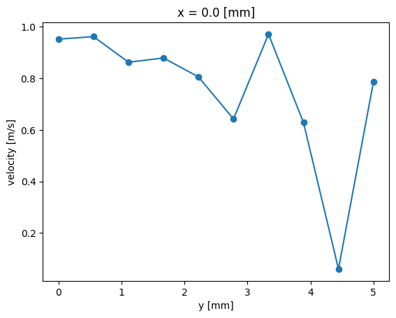
Line plots

with h5tbx.File(h5.hdf_filename) as h5:
    h5.dump()
    d = h5['data'][:, 0]
    d.plot.line(marker='o')

• /(8)
  data (y: 10, x: 20) [float64]
  • long_name : velocity
  • units : m/s
  u (z: 4, y: 10, x: 20) [float64]
  • long_name : x_velocity
  • units : m/s
  v (z: 4, y: 10, x: 20) [float64]
  • long_name : y_velocity
  • units : m/s
  w (z: 4, y: 10, x: 20) [float64]
  • long_name : z_velocity
  • units : m/s
  x (20) [float64]
  • long_name : x
  • units : mm
  y (10) [float64]
  • long_name : y
  • units : mm
  z (4) [float64]
  • long_name : z
  • units : mm
  • h5rdmtoolbox @type: https://schema.org/SoftwareSourceCode(0)
    • __h5rdmtoolbox_version__ https://schema.org/softwareVersion : 1.2.3a2
    • codeRepository https://schema.org/codeRepository : https://github.com/matthiasprobst/h5RDMtoolbox

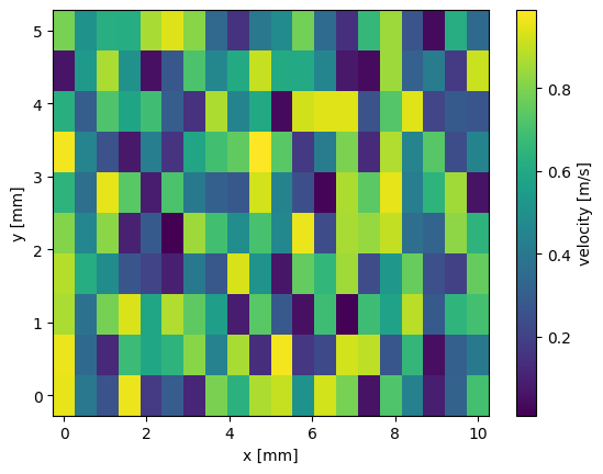
2D plots

with h5tbx.File(h5.hdf_filename) as h5:
    # some plotting
    plt.figure()
    h5['data'][:].plot()
    plt.show()
    
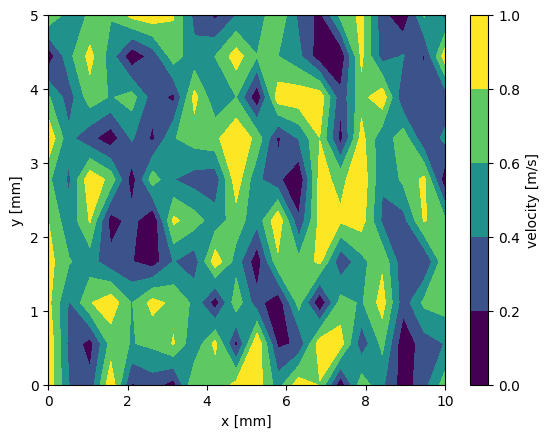
    plt.figure()
    h5['data'][:].plot.contourf()
    plt.figure()
    plt.show()

<Figure size 640x480 with 0 Axes>

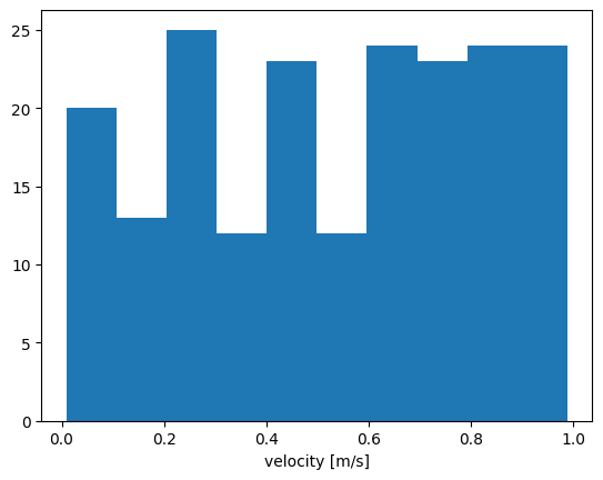
Histograms

with h5tbx.File(h5.hdf_filename) as h5:
    h5['data'][:].plot.hist()
    plt.show()

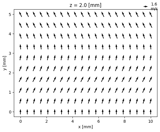
Vector plotting with h5rdmtoolbox and xarray

The toolbox provides a Vector accessory (see also section Extensions)), which constructs a xarray dataset:

from h5rdmtoolbox.extensions import vector
with h5tbx.File(h5.hdf_filename) as h5:
    ds = h5.Vector(u=h5.u, v=h5.v)
    ds[2, :, :].plot.quiver(x='x', y='y', u='u', v='v')